A more flexible LCM - beta version
As mentionneed in this post, we are looking for a new closed itemset mining algorithm, with a lightweight design.
In this post we will discuss about data structures, and the improvements we can leverage thanks to these structs.
Roaring Bitmaps
The first structs we are going to extensively use are RoaringBitmaps.
RoaringBitmaps are compressed implementations of bitmaps. They allow peformant
operations, going way faster than the classic set (or frozenset) struct in Python,
and consuming orders of magnitude less memory.
There are a few implementations of those bitmaps in Python, mostly providing the same order of performance on the main operations (issubset, and, xor, …), but I settled for this implemenation in Cython, considering the variety of functions accessible through the API
As an example, because of the way roaring bitmaps are made, we don’t need to actually compute the intersection between two bitmaps to compute the length of this intersection. Instead of doing
len(bitmap_1.intersection(bitmap_2)) # compute the intersection, store it, return lenWe will do
bitmap_1.intersection_len(bitmap_2) # compute the intersection len, store it as an uintBeta design of the algorithm
We will take a simple use case : a set of 7 transactions. Then we insert them into
the item_to_tids : a dictionnary keeping track of every item, and the transaction ids for these items
>>> transactions = [
>>>    [1, 2, 3, 4, 5, 6],
>>>    [2, 3, 5],
>>>    [2, 5],
>>>    [1, 2, 4, 5, 6],
>>>    [2, 4],
>>>    [1, 4, 6],
>>>    [3, 4, 6],
>>>]

>>> lcm = LCM(min_supp=3)

>>> for t in transactions:
>>>     lcm.add(t)

>>> lcm.item_to_tids
{1: RoaringBitmap({0, 3, 5}),
 2: RoaringBitmap({0, 1, 2, 3, 4}),
 3: RoaringBitmap({0, 1, 6}),
 4: RoaringBitmap({0, 3, 4, 5, 6}),
 5: RoaringBitmap({0, 1, 2, 3}),
 6: RoaringBitmap({0, 3, 5, 6})}
Main function
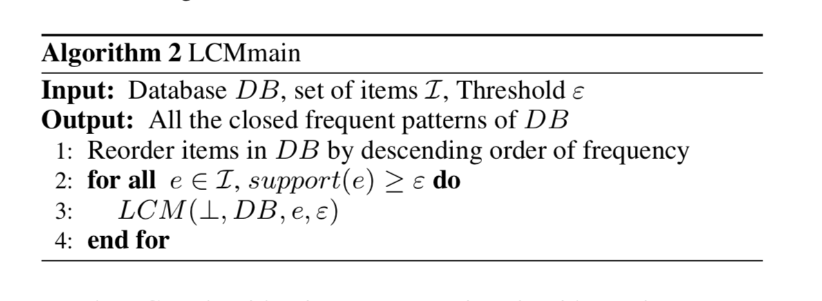
For the main part, we keep it the same way as in the original
HLCM paper. Only the LCM function will change (line 3)
LCM function
Below is a compaison between the original inner algorithm as described in the paper and my implemenation.
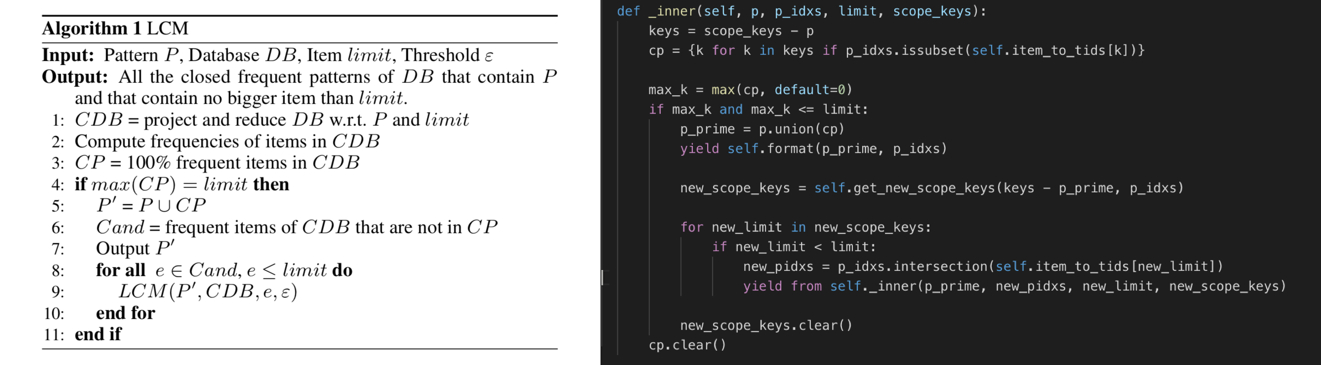
Main modifications
- We do not have a CDB anymore (line 1). Instead we use RoaringBitmaps to find every item which transactions ids are subsets of the current itemset’s transaction ids. As a result, we get the exact same set of items that in the original paper
- The
get_new_scope_keysfunction make several calls toRoaringBitmap.intersection_len, and corresponds toCandin the paper (line 6)
Profiling (with line_profiler) and future work
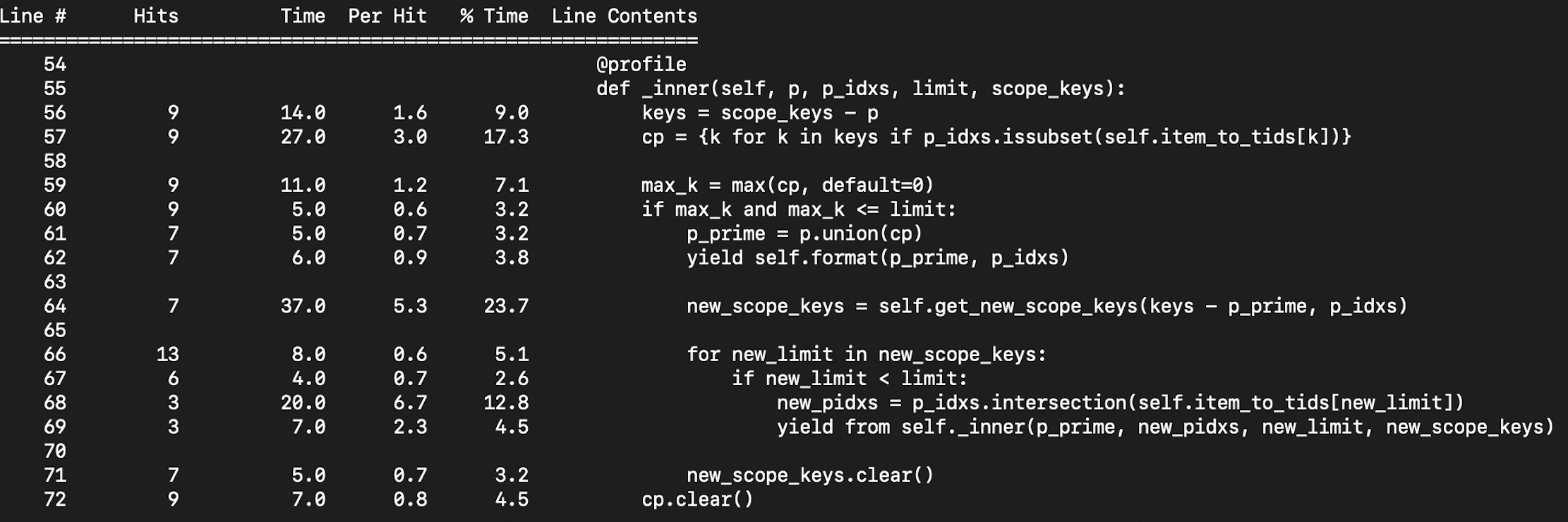
Here is a line profiling of the algorithm, runned on the transactions we used up until now. A few additional informations before rushing into conclusions:
cpis computed 9 times (line 57) because we have a 6 distinct items in our transactions, and we go 3 times into recursion (line 71).self.formatdoes nothing but yielding (p_prime, len(p_idxs)), as the length of p_idxs is the support for p_prime
Now concerning the profiling in itself :
- 20% of the time is spent on computing
cp. Even if calls toissubsetare really fast thaks to RoaringBitmaps, we just go over the entire set of keys to compute cp, which is far from optimal. We can certainly do better. - 8% of the time comes from calls to max. This should be independant from the computation of
cp, so we cannot realy expect any speedup on this part. - 20 % of the time is spent computing the new keys
(
new_scope_keysin my implementation,Candin the paper)
As we have seen, the main bottle neck is on cp computation. Even with a small data
example like the one above we can conclude that it is not acceptable to iterate
over the complete set of keys eveytime we need a new cp.
In a next post we will use sorted data structures, in order to make strong assumptions on our
set of items, and reduce time complexity for the pain points mentioned above